Have you ever heard someone (mostly Product managers) saying ‘We ran an experiment to validate the hypothesis X, and we have reached the conclusion Y. We are pretty confident about this because we have statistically significant data on this experiment’, and wondered ‘how do they know that the data they have is statistically significant?’. Also, the next obvious question would be ‘How likely is that the assumption is correct?’

Is it the sheer amount of data that dictates this, or is it something else?

In this article, I’ll try to explain when can we claim if we have statically significant data. This will not only help us to be confident in our conclusions, but we can even articulate and say ‘There is a 99.7% chance that our hypothesis is correct’. Sounds interesting? Then carry along!

Statistics sometimes seem like magic. We can make sweeping conclusions about a population with the help of just a few amount of data. This power of inference is truly great since we can’t have data of an entire population. Where does this power come from? or, when do we know that the information we have from a small set of data, can truly be conclusive? The answer is, in major parts due to The Central Limit Theorem.

The Central Limit Theorem

The main idea of the central limit theorem is pretty simple. It basically says that a large, properly drawn sample will resemble the population from which it was drawn. There will a little variation from sample to sample, but it’s very unlikely that the variation will deviate massively from the underlying population.

Example

Imagine you are observing 1000 male Olympic runners. If you take a sample of random 100 runners from that crowd, you’d find the mean of those 100 runners close to the mean of 1000 runners (since they should be more or less similar physically). No matter who you choose in the sample. Sure, there may be a slight variation in the means, but the average would most likely be closer to the population’s average (If you have noticed already, this can be called a properly drawn sample since the sample we are taking is reflective of the population.)

Let’s turn things around. The beauty of the central limit theorem is that, if you had taken an average of random 100 runners from the population, you could’ve made a strikingly accurate inference about the mean weight of the population, even though you didn’t have to measure the weight of each of the 1000 runners!

From one of the well-written books on statistics, Naked Statistics by Charles Wheelan:

Of course, this is how polling works. A methodologically sound poll of 1,200 Americans can tell us a great deal about how the entire country is thinking.

Not only the central limit theorem allows you to make a pretty accurate estimate about the underlying population from just a sample, it goes beyond that, and can assign a degree of confidence to the conclusion.

The Central limit theorem tells us that the sample mean will be distributed as normal distribution around the population mean. (as shown in the image below) 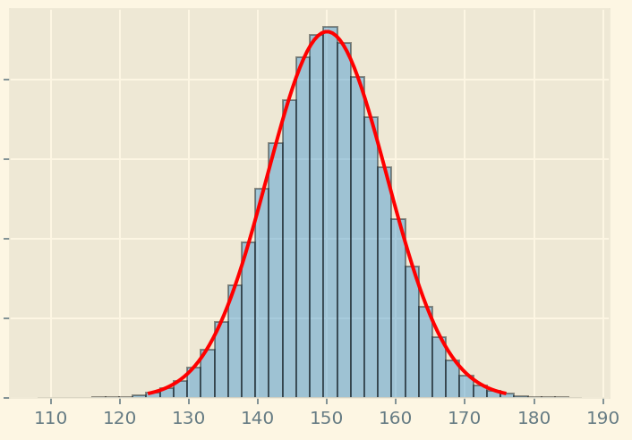Some sample means may be a little higher, or a little lower, very few will either be significantly lower, or significantly higher. The key point is that they will always form a normal distribution (like the above symmetric image). This is true no matter what the distribution of the underlying population is (I know I took an example of runners which are most likely to have the same phyical weight, but the theorem works on any kind of distribution). Here’s another image that depicts that: 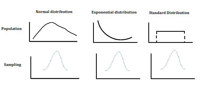No matter how the weigh is distributed among the population, you’ll always reach a normal distribution after sampling.

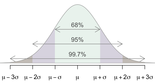
Now the time of big reveal. Since the sample means will be distributed as a normal distribution, 68% of the observation will lie within one standard deviation of the mean, 95% within the two standard deviations, and 99.7% within 3 standard deviations (If mean gives us the average of data points, standard deviation tells us how spread the data points are).

But what does that mean actually? Let’s pull out the sample mean distribution we used before: Imagine in the above graph, the standard error (Don’t get confused here. Standard error is ‘kind-of’ like standard deviation. Just like standard deviation measures the dispersion of weights of all participants, standard error measures the dispersion of the sample mean) is 10 pounds. Now with the insight, we uncovered before, If some random person (let’s name him Kyle) say ‘Hey, the sample mean of 100 people is 185 pounds’, then we can say that ‘We are 99.7% sure that the sample Kyle has collected does not belong to the 100 runners’.

See what I did there? With the help of the central limit theorem, not only we can judge a hypothesis, whether it’s true or false, we can also assign a degree of confidence to our claim. How could we say that? Since the mean of the 100 athletes was 150 pounds, the standard error is 10 pound, the sample mean of some random population (might not be even of athletes, but could be of sumo-wrestlers) given by the our friend Kyle is 185 pound, which is 3 standard errors ahead of the mean. Since we know 99.7% percent of observation lie within 3 standard deviations of the mean, we are 99.7% sure that the sample Kyle has doesn’t belong to the athlete group.

Time for some jargons:

• Null hypothesis: This is our starting hypothesis about anything, which can be accepted or refuted based on statistical analysis. In the above example, Kyle’s ‘The sample mean of 100 Olympic athlets is 185 pound’ was a null hypothesis. Think of this as simply a hypothesis under test. Another example: ‘Adding song and dance above the ‘Buy Now’ button will improve the number of sales’

• Significance level: A common threshold for rejecting a null hypothesis is 5%, which is often written as 0.05 in decimal. This is what a significance level is. In the above example, suppose the null hypothesis had instead said ‘The sample mean of 100 Olympic athlets is 175 pound’. Since 175 pounds is 2 standard deviations away in the graph, and we know 95% of observations lie within 2 standard deviations in a normal distribution, we can reject the null hypothesis with a significance level of 0.05, if there is less than 5% chance of getting an outcome as extreme as this.

When we reject a null hypothesis at some reasonable significance level, the results are said to be statistically significant

More on the Significance level

Now the obvious question lingering in your mind is ‘How to know which significance level is the best?’. There is no right answer to it, and significance levels have trade-offs. Imagine if we take a high significance level, i.e. p = 0.1, we’ll be rejecting the null hypothesis fairly often which in fact might be true. Here’s a well put excerpt from the book Naked Statistics by Charles Wheelan:

Consider the example of an American courtroom, where the null hypothesis is that a defendant is not guilty and the threshold for rejecting that null hypothesis is “guilty beyond a reasonable doubt.” Suppose we were to relax that threshold to something like “a strong hunch that the guy did it.” This is going to ensure that more criminals go to jail—and also more innocent people. In a statistical context, this is the equivalent of having a relatively low significance level, such as .1. This happens because 1 in 10 is not very improbable. 10 miracle drugs are created, and 1 might show favorable results just by chance.

Now let’s see the other extreme. Imagine we choose a very high significance level i.e. p = 0.001. This will be the equivalent of requiring 5 eye-witnesses for every criminal defendant to prove him guilty. If we apply this to drug discovery, we will indeed minimize the approval of ineffective drugs, but we’d see a decline in the approval of quite-effective drugs because we set the bar so high.

Gotchas:

• For the Central limit theorem to work properly, the sample size should be atleast 30.

• Significance test is good for accepting and rejecting the null hypothesis, but it isn’t perfect. It can tell you that adding dance and music to ‘Buy Now’ button does have a significant effect on the purchase. But it won’t tell you how big the effect will be. 10% more sales? 50% more sales? It just won’t tell you that.

• It’s imperative that the data you have isn’t inherently biased. Either directly or indirectly.

“Most statistics books assume that you are using good data, just as a cookbook assumes that you are not buying rancid meat and rotten vegetables. But even the finest recipe isn’t going to salvage a meal that begins with spoiled ingredients”

I wrote a piece ‘Garbage in, Garbage out: Hidden biases in data’ which goes in the detail of that issue. Feel free to check that out.

Resources:

How to Lie with Statistics By D. Huff,I. Geis

Naked Statistics: Stripping the Dread from the Data

Youtube video on Standard Deviation